
Example
This example illustrates the analysis steps the AMIA Toolbox performs when finding and characterizing the spots in a microarray image. More detailed information is available in the documentation included with the toolbox.
The original slide image is dark, with only a few visible spots (Figure 1).
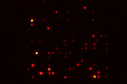
Figure 1: Original microarray slide image
The AMIA tool first contrast-enhances the image to enable identification of the spots (Figure 2). The enhanced image is only used for spot identification, not for spot characterization.
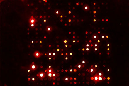
Figure 2: Contrast-enhanced slide image used for spot identification
Using the enhanced image, initial spot center estimates are created (Figure 3). On the first image in a collection, these initial estimates are created by prompting the user for information. This grid of spot centers is saved and applied automatically to the subsequent slides.

Figure 3: Initial spot center estimates
The typical spot size and shape is estimated from the brightest spots on the slide (Figure 4).
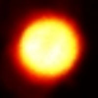

Figure 4: Typical spot (left) and estimated spot size and shape (right)
This fixed spot is combined with the expected spot centers to create the ideal spot map, which assumes identically shaped spots in a perfect grid (Figure 5).
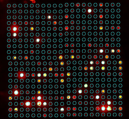
Figure 5: Ideal spot map (spot outlines)
This ideal spot map provides a basis for two more adaptive spot identification methods. The first assumes a fixed spot shape as before, but allows the spot centers to vary within a small region around the expected location (Figure 6). This allows for small variations in printing.
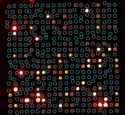
Figure 6: Spot map with fixed spot shape, but variable centers
The final spot finding method uses a seeded region growing algorithm to identify only the pixels that are sufficiently different from the background (Figure 7). Thus only spots that have reacted will be found. This allows the spots to assume any shape, but the algorithm may also identify smears or streaks on the slide due to the lack of constraints on size and shape.
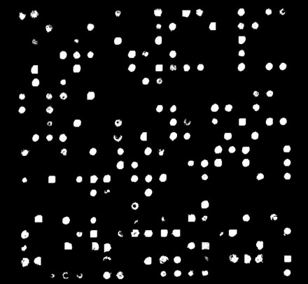
Figure 7: Seeded-region grower spot map
Summary and diagnostic statistics are calculated for the spots for each method of identification, thus three full sets of statistics are output. It is up to the user to determine which set of statistics they want to use.
These statistics include the typical spot mean, median and standard deviation, along with background intensity and standard deviation. Also included are size and shape statistics. These are particularly crucial for the seeded region grower spots to eliminate cases where the algorithm has identified streaks, scratches or other non-spots.
All of these images are displayed in an HTML browser interface, along with other diagnostic images and statistics. These include analysis of background over the slide, to identify if there is uneven background and a comparison of local background to spot intensity, which identifies if there is a spot overshine problem.